Customers-Segmentation-with-RFM
- 19 minsCustomers-Segmentation-with-RFM

RFM Segmentation
- The RFM method was introduced by Bult and Wansbeek in 1995 and has been successfully used by marketers since.
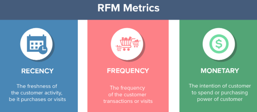
- It analyzes customers’ behavior on three parameters:
- Recency: How recent is the last purchase of the customer.
- Frequency: How often the customer makes a purchase.
- Monetary: How much money does the customer spends.
- RFM Analysis is a technique used to segment customer behavior. RFM is a data science analytics application.
- It is a rule-based method, not a machine learning model.
- It helps to determine marketing and sales strategies based on customers’ purchasing habits.
Advantages & Disadvantages
-
The advantages of RFM is that it is easy to implement and it can be used for different types of business. It helps craft better marketing campaigns and improves CRM and customer’s loyalty.
-
The disadvantages are that it may not apply in industries where customers are usually one time buyers. It is based on historical data and won’t give much insight about prospects.
RFM Metrics
Recency Calculation
We create the recency (R) variable from the date variable we have. What we do is to subtract the last shopping date of each customer from the specified last shopping day.
Here, the perception of size and smallness is different for the Recency score. That is, a value of 1 for Recency (last shopped 1 day ago) is the best value for us, while a value of 80 is worse than 1.
Frequency Calculation
Frequency (F) consists of the total number of purchases made by each customer.
The point to be noted here is that each unique invoice number can be multiplexed and we need to count it as singular.
Monetary Calculation
In the Monetary (M) part, we calculate the money that the customer earns for us in this time period.
In our sample dataset, there was no such variable that we could take directly, and we calculated the total amount of each purchase by multiplying the number of products with the unit prices.
Methodology
To get the RFM score of a customer, we need to first calculate the R, F and M scores on a scale from 1 (worst) to 5 (best).
- calculate Recency = number of days since last purchase
- calculate Freqency = number of purchases during the studied period (usually one year)
- calculate Monetary = total amount of purchases made during the studied period
- find quintiles for each of these dimensions
- give a grade to each dimension depending in which quintiles it stands
- combine R, F and M scores to get the RFM score
- map RF scores to segments
For this example, I will use the Online Retail dataset.
We have a Bussines problem.
- An e-commerce company segments its customers and determine marketing strategies according to segments wants.
- Customer segments with common behaviors Income increase by doing marketing studies in particular thinks it will.
- For example, retaining customers that are very lucrative for the company different campaigns for new customers. Campaigns are wanted.
Dataset Story
- The dataset named Online Retail II is a UK-based online sales company. Store’s sales between 01/12/2009 - 09/12/2011 contains.
- The product catalog of this company includes souvenirs.
- The vast majority of the company’s customers are corporate customers.
RESOURCES AND THANKS
Let’s move on to our example

Necessary Import
!pip install openpyxl
import datetime as dt
import pandas as pd
import matplotlib.pyplot as plt
Collecting openpyxl
Downloading openpyxl-3.0.9-py2.py3-none-any.whl (242 kB)
|████████████████████████████████| 242 kB 288 kB/s
[?25hCollecting et-xmlfile
Downloading et_xmlfile-1.1.0-py3-none-any.whl (4.7 kB)
Installing collected packages: et-xmlfile, openpyxl
Successfully installed et-xmlfile-1.1.0 openpyxl-3.0.9
[33mWARNING: Running pip as the 'root' user can result in broken permissions and conflicting behaviour with the system package manager. It is recommended to use a virtual environment instead: https://pip.pypa.io/warnings/venv[0m
df_ = pd.read_excel("../input/online-retail-ii/online_retail_II.xlsx", sheet_name="Year 2010-2011")
df = df_.copy()
df.head()
| Invoice | StockCode | Description | Quantity | InvoiceDate | Price | Customer ID | Country | |
|---|---|---|---|---|---|---|---|---|
| 0 | 536365 | 85123A | WHITE HANGING HEART T-LIGHT HOLDER | 6 | 2010-12-01 08:26:00 | 2.55 | 17850.0 | United Kingdom |
| 1 | 536365 | 71053 | WHITE METAL LANTERN | 6 | 2010-12-01 08:26:00 | 3.39 | 17850.0 | United Kingdom |
| 2 | 536365 | 84406B | CREAM CUPID HEARTS COAT HANGER | 8 | 2010-12-01 08:26:00 | 2.75 | 17850.0 | United Kingdom |
| 3 | 536365 | 84029G | KNITTED UNION FLAG HOT WATER BOTTLE | 6 | 2010-12-01 08:26:00 | 3.39 | 17850.0 | United Kingdom |
| 4 | 536365 | 84029E | RED WOOLLY HOTTIE WHITE HEART. | 6 | 2010-12-01 08:26:00 | 3.39 | 17850.0 | United Kingdom |
Task 1
Understanding and Preparing Data
Let’s examine the descriptive statistics of the dataset
df.shape
(541910, 8)
df.columns
Index(['Invoice', 'StockCode', 'Description', 'Quantity', 'InvoiceDate',
       'Price', 'Customer ID', 'Country'],
      dtype='object')
df.describe().T
| count | mean | std | min | 25% | 50% | 75% | max | |
|---|---|---|---|---|---|---|---|---|
| Quantity | 541910.0 | 9.552234 | 218.080957 | -80995.00 | 1.00 | 3.00 | 10.00 | 80995.0 |
| Price | 541910.0 | 4.611138 | 96.759765 | -11062.06 | 1.25 | 2.08 | 4.13 | 38970.0 |
| Customer ID | 406830.0 | 15287.684160 | 1713.603074 | 12346.00 | 13953.00 | 15152.00 | 16791.00 | 18287.0 |
Are there any missing observations in the dataset? If yes, how many missing observations in which variable?
df.isnull().sum()
Invoice             0
StockCode           0
Description      1454
Quantity            0
InvoiceDate         0
Price               0
Customer ID    135080
Country             0
dtype: int64
Let’s remove the missing observations from the data set
df.dropna(inplace=True)
What is the number of unique products?
df.Description.nunique()
3896
How many of each product are there?
df.Description.value_counts().head(10)
WHITE HANGING HEART T-LIGHT HOLDER    2070
REGENCY CAKESTAND 3 TIER              1905
JUMBO BAG RED RETROSPOT               1662
ASSORTED COLOUR BIRD ORNAMENT         1418
PARTY BUNTING                         1416
LUNCH BAG RED RETROSPOT               1358
SET OF 3 CAKE TINS PANTRY DESIGN      1232
POSTAGE                               1197
LUNCH BAG  BLACK SKULL.               1126
PACK OF 72 RETROSPOT CAKE CASES       1080
Name: Description, dtype: int64
Let’s sort the 5 most ordered products from most to least
df.groupby("Description").agg({"Quantity": "sum"}).sort_values("Quantity", ascending=False).head()
| Quantity | |
|---|---|
| Description | |
| WORLD WAR 2 GLIDERS ASSTD DESIGNS | 53215 |
| JUMBO BAG RED RETROSPOT | 45066 |
| ASSORTED COLOUR BIRD ORNAMENT | 35314 |
| WHITE HANGING HEART T-LIGHT HOLDER | 34147 |
| PACK OF 72 RETROSPOT CAKE CASES | 33409 |
The ‘C’ in the invoices shows the canceled transactions. Let’s remove the canceled transactions from the dataset.
df = df[~df["Invoice"].astype(str).str.contains("C", na=False)]
df.head()
| Invoice | StockCode | Description | Quantity | InvoiceDate | Price | Customer ID | Country | |
|---|---|---|---|---|---|---|---|---|
| 0 | 536365 | 85123A | WHITE HANGING HEART T-LIGHT HOLDER | 6 | 2010-12-01 08:26:00 | 2.55 | 17850.0 | United Kingdom |
| 1 | 536365 | 71053 | WHITE METAL LANTERN | 6 | 2010-12-01 08:26:00 | 3.39 | 17850.0 | United Kingdom |
| 2 | 536365 | 84406B | CREAM CUPID HEARTS COAT HANGER | 8 | 2010-12-01 08:26:00 | 2.75 | 17850.0 | United Kingdom |
| 3 | 536365 | 84029G | KNITTED UNION FLAG HOT WATER BOTTLE | 6 | 2010-12-01 08:26:00 | 3.39 | 17850.0 | United Kingdom |
| 4 | 536365 | 84029E | RED WOOLLY HOTTIE WHITE HEART. | 6 | 2010-12-01 08:26:00 | 3.39 | 17850.0 | United Kingdom |
We want the Quentity and Price variables to be greater than 0
df = df[(df['Quantity'] > 0)]
df = df[(df['Price'] > 0)]
Let’s create a variable called ‘TotalPrice’ that represents the total earnings per invoice
df["TotalPrice"] = df["Quantity"] * df["Price"]
Task 2
Calculating RFM metrics
df["InvoiceDate"].max()                  # Timestamp('2011-12-09 12:50:00')   we look at the date of the last invoice transaction
                                         # Because we will determine the date when we will do our analysis.
today_date = dt.datetime(2011, 12, 11)   # We determine the date of the analysis
rfm = df.groupby('Customer ID').agg({'InvoiceDate': lambda InvoiceDate: (today_date - InvoiceDate.max()).days, # recency
                                     'Invoice': lambda Invoice: Invoice.nunique(),                             # frequency
                                     'TotalPrice': lambda TotalPrice: TotalPrice.sum()})                       # monetary
rfm.head()
rfm.columns = ['recency', 'frequency', 'monetary'] # updating our variable names
rfm = rfm[rfm["monetary"] > 0] # We filter out winners with more than 0
Task 3
Generating RFM scores
rfm["recency_score"] = pd.qcut(rfm["recency"], 5, labels=[5,4,3,2,1])
rfm["frequency_score"] = pd.qcut(rfm["frequency"].rank(method="first"),5,labels=[1,2,3,4,5,])
rfm["monetary_score"] = pd.qcut(rfm["monetary"],5, labels=[1,2,3,4,5])
rfm["RFM_SCORE"] = (rfm["recency_score"].astype(str)+rfm["frequency_score"].astype(str))
# We did not consider Monetary because we will do a segmentation operation. We calculate this process over recency and frequency.
Task 4
Defining RFM scores as segments
seg_map = {
    r'[1-2][1-2]': 'hibernating',
    r'[1-2][3-4]': 'at_Risk',
    r'[1-2]5': 'cant_loose',
    r'3[1-2]': 'about_to_sleep',
    r'33': 'need_attention',
    r'[3-4][4-5]': 'loyal_customers',
    r'41': 'promising',
    r'51': 'new_customers',
    r'[4-5][2-3]': 'potential_loyalists',
    r'5[4-5]': 'champions'
}
rfm["SEGMENT"] = rfm["RFM_SCORE"].replace(seg_map,regex=True)
rfm.head()
| recency | frequency | monetary | recency_score | frequency_score | monetary_score | RFM_SCORE | SEGMENT | |
|---|---|---|---|---|---|---|---|---|
| Customer ID | ||||||||
| 12346.0 | 326 | 1 | 77183.60 | 1 | 1 | 5 | 11 | hibernating |
| 12347.0 | 3 | 7 | 4310.00 | 5 | 5 | 5 | 55 | champions |
| 12348.0 | 76 | 4 | 1797.24 | 2 | 4 | 4 | 24 | at_Risk |
| 12349.0 | 19 | 1 | 1757.55 | 4 | 1 | 4 | 41 | promising |
| 12350.0 | 311 | 1 | 334.40 | 1 | 1 | 2 | 11 | hibernating |
Task 5
Action Time
- Let’s choose 3 segments that we find important. These three segments;
- Both in terms of action decisions,
- Both in terms of the structure of the segments (mean RFM values) let’s comment.
rfm[["SEGMENT", "recency", "frequency", "monetary"]].groupby("SEGMENT").agg(["mean", "count","max"])
| recency | frequency | monetary | |||||||
|---|---|---|---|---|---|---|---|---|---|
| mean | count | max | mean | count | max | mean | count | max | |
| SEGMENT | |||||||||
| about_to_sleep | 53.312500 | 352 | 72 | 1.161932 | 352 | 2 | 471.994375 | 352 | 6207.67 |
| at_Risk | 153.785835 | 593 | 374 | 2.876897 | 593 | 6 | 1084.535297 | 593 | 44534.30 |
| cant_loose | 132.968254 | 63 | 373 | 8.380952 | 63 | 34 | 2796.155873 | 63 | 10254.18 |
| champions | 6.361769 | 633 | 13 | 12.413902 | 633 | 209 | 6857.963918 | 633 | 280206.02 |
| hibernating | 217.605042 | 1071 | 374 | 1.101774 | 1071 | 2 | 488.643307 | 1071 | 77183.60 |
| loyal_customers | 33.608059 | 819 | 72 | 6.479853 | 819 | 63 | 2864.247791 | 819 | 124914.53 |
| need_attention | 52.427807 | 187 | 72 | 2.326203 | 187 | 3 | 897.627861 | 187 | 12601.83 |
| new_customers | 7.428571 | 42 | 13 | 1.000000 | 42 | 1 | 388.212857 | 42 | 3861.00 |
| potential_loyalists | 17.398760 | 484 | 33 | 2.010331 | 484 | 3 | 1041.222004 | 484 | 168472.50 |
| promising | 23.510638 | 94 | 33 | 1.000000 | 94 | 1 | 294.007979 | 94 | 1757.55 |
rfm["SEGMENT"].value_counts().plot(kind='barh', rot=5, fontsize=20)
plt.show()
MY SELECTED SEGMENTS AND ACTION SUGGESTIONS
champions Champions. They want to listen to champions league music all the time. they’re like haalaand who even set their alarms to this music on their phones.
- Our best customers are in this group.
- It consists of the group whose last shopping dates are the closest and who visit us most frequently.
- As an average of us; They earned 6857.96392 units of money
- Frequency of visits 12,41390
- They last shopped 6.36177 days ago.
rfm[rfm["SEGMENT"] == "champions"].head()
| recency | frequency | monetary | recency_score | frequency_score | monetary_score | RFM_SCORE | SEGMENT | |
|---|---|---|---|---|---|---|---|---|
| Customer ID | ||||||||
| 12347.0 | 3 | 7 | 4310.00 | 5 | 5 | 5 | 55 | champions |
| 12362.0 | 4 | 10 | 5226.23 | 5 | 5 | 5 | 55 | champions |
| 12364.0 | 8 | 4 | 1313.10 | 5 | 4 | 4 | 54 | champions |
| 12381.0 | 5 | 5 | 1845.31 | 5 | 4 | 4 | 54 | champions |
| 12417.0 | 4 | 9 | 3649.10 | 5 | 5 | 5 | 55 | champions |
rfm[rfm["SEGMENT"] == "champions"].describe().T
| count | mean | std | min | 25% | 50% | 75% | max | |
|---|---|---|---|---|---|---|---|---|
| recency | 633.0 | 6.361769 | 3.683300 | 1.00 | 3.00 | 5.00 | 10.00 | 13.00 |
| frequency | 633.0 | 12.413902 | 16.451672 | 3.00 | 5.00 | 8.00 | 14.00 | 209.00 |
| monetary | 633.0 | 6857.963918 | 20339.763842 | 201.12 | 1451.28 | 2612.96 | 4954.84 | 280206.02 |
Action Suggestions
- When we add new products to our catalog » let’s send a message saying “hello handsome/beautiful I have something new for you”
- will apply a discount from us to their last purchase when they reach the specific purchase. »
-
If they bring us new customers, we can prepare special campaigns for them »
loyal_customers Our loyal friends. They are in the 2nd most traded group but one of the most precious to us. In an important situation, they can be our airbag.
- So they seem to have certain habits we can trust.
- As an average of us; They earned 2864.24779 units of money
- Frequency of visits 6.47985
- They last shopped 33,60806 days ago.
rfm[rfm["SEGMENT"] == "loyal_customers"].head()
| recency | frequency | monetary | recency_score | frequency_score | monetary_score | RFM_SCORE | SEGMENT | |
|---|---|---|---|---|---|---|---|---|
| Customer ID | ||||||||
| 12352.0 | 37 | 8 | 2506.04 | 3 | 5 | 5 | 35 | loyal_customers |
| 12359.0 | 58 | 4 | 6372.58 | 3 | 4 | 5 | 34 | loyal_customers |
| 12370.0 | 52 | 4 | 3545.69 | 3 | 4 | 5 | 34 | loyal_customers |
| 12380.0 | 22 | 4 | 2724.81 | 4 | 4 | 5 | 44 | loyal_customers |
| 12388.0 | 16 | 6 | 2780.66 | 4 | 4 | 5 | 44 | loyal_customers |
rfm[rfm["SEGMENT"] == "loyal_customers"].describe().T
| count | mean | std | min | 25% | 50% | 75% | max | |
|---|---|---|---|---|---|---|---|---|
| recency | 819.0 | 33.608059 | 15.577050 | 15.00 | 20.000 | 30.00 | 44.000 | 72.00 |
| frequency | 819.0 | 6.479853 | 4.545669 | 3.00 | 4.000 | 5.00 | 8.000 | 63.00 |
| monetary | 819.0 | 2864.247791 | 6007.061883 | 36.56 | 991.795 | 1740.48 | 3052.905 | 124914.53 |
Action Suggestions
- We can define short-term discounts on the products they buy most often
-
If they bring us new customers, we can prepare special campaigns for them
at risk Woowo we haven’t seen these friends for a long time, let’s get their attention a little bit
- As an average of us; They earned 1084.53530 units of money
- Frequency of visits 2.87858
- They last shopped 153.78583 days ago.
rfm[rfm["SEGMENT"] == "at_Risk"].head()
| recency | frequency | monetary | recency_score | frequency_score | monetary_score | RFM_SCORE | SEGMENT | |
|---|---|---|---|---|---|---|---|---|
| Customer ID | ||||||||
| 12348.0 | 76 | 4 | 1797.24 | 2 | 4 | 4 | 24 | at_Risk |
| 12383.0 | 185 | 5 | 1850.56 | 1 | 4 | 4 | 14 | at_Risk |
| 12393.0 | 73 | 4 | 1582.60 | 2 | 4 | 4 | 24 | at_Risk |
| 12399.0 | 120 | 4 | 1108.65 | 2 | 4 | 4 | 24 | at_Risk |
| 12409.0 | 79 | 3 | 11072.67 | 2 | 3 | 5 | 23 | at_Risk |
rfm[rfm["SEGMENT"] == "at_Risk"].describe().T
| count | mean | std | min | 25% | 50% | 75% | max | |
|---|---|---|---|---|---|---|---|---|
| recency | 593.0 | 153.785835 | 68.618828 | 73.0 | 96.00 | 139.00 | 195.00 | 374.0 |
| frequency | 593.0 | 2.876897 | 0.951540 | 2.0 | 2.00 | 3.00 | 3.00 | 6.0 |
| monetary | 593.0 | 1084.535297 | 2562.073355 | 52.0 | 412.78 | 678.25 | 1200.62 | 44534.3 |
Action Suggestions
- “Hey “NAME” sir/ma’am, we missed you so much. Let’s send you an e-mail if you want to take a look at our special offers.
- They didn’t bring us bad income. Let’s remind ourselves of them. We can inform you about existing campaigns.